Water Quality Statistics
We developed a series of linear mixed effects models to estimate concentrations for constituents of concern (COCs) in Puget Sound urban stormwater. Spatial covariates in the models included various landscape predictors, rainfall, seasonal components, and in some models, percent land use (commercial, industrial, residential).
Data Sources
Outfall Data
The primary source of measured stormwater data is the S8.D Municipal Stormwater Permit Outfall Data (referred to as the S8 Data in this document) provided by the Washington Department of Ecology (Hobbs et al., 2015). Special Condition S8.D of the 2007-2012 Phase I Municipal Stormwater Permit required permittees to collect and analyze data to evaluate pollutant loads in stormwater discharged from different land uses: high density (HD) residential, low density (LD) residential, commercial, and industrial. Phase I Permittees[1] collected water quality and flow data, sediment data, and toxicity information from stormwater discharges during storm events. Stormwater data collected from a total of 16 outfalls by six Phase I Permittees was utilized in this modeling study.
The stormwater outfall data are available from Ecology via an open-data api at: https://data.wa.gov/Natural-Resources-Environment/Municipal-Stormwater- Permit-Outfall-Data/d958-q2ci.
COCs analyzed in this study are:
-
Copper – Total
-
Total Suspended Solids (TSS)
-
Phosphorus – Total
-
Zinc - Total
-
Total Kjeldahl Nitrogen (TKN)
We extracted data for these COCs, and performed minimal data cleaning. We filtered out rejected data (values with a R or REJ flag), removed replicates, and removed one data point for TKN that was an outlier (an order of magnitude higher than the majority of the data). Figure 4.1 shows data before removal of the outlier.
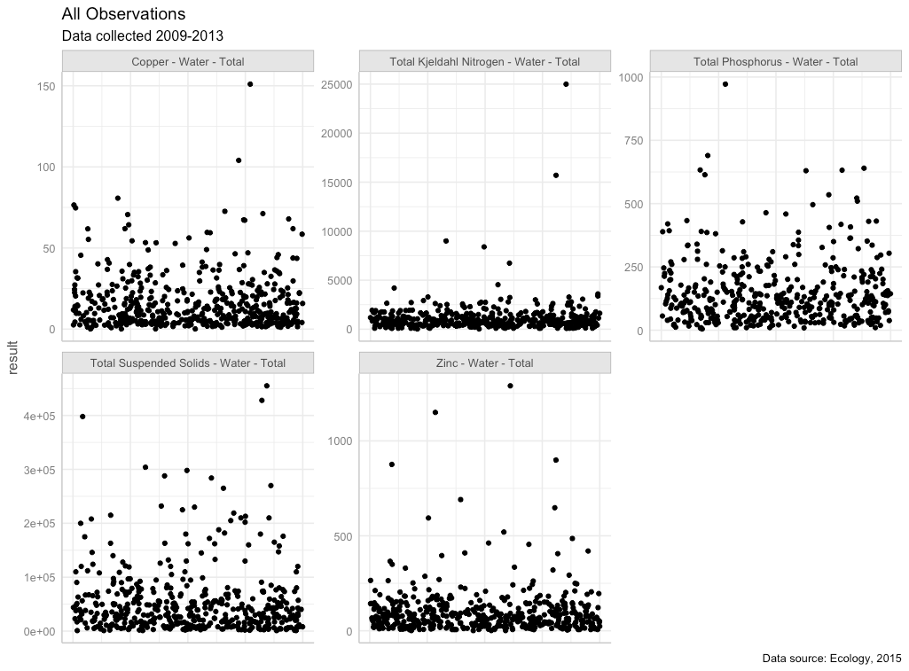
Figure 4.1 All observations with outlier in place for Total Kjeldahl nitrogen (TKN)
Censored (Non-Detect) Data
Nearly all COCs had non-detect (left-censored) data present (Table 4.1). Ecology flagged non-detect data and provided the reporting limit for each non-detect value. Most COCs had a very small percentage of data that were non-detect (2% or less); one COC, TKN, had a higher level of non-detect data (just over 10%). For all COCs, non-detect values were substituted with one-half of the reporting limit. Models using censored methods were compared to linear models for TKN to verify that data substitution on linear mixed effects models generated suitable results.
Table 4.1 Percentage of data points that were left-censored (non-detect) for each chemical of concern
| C hemical of Concern | Ce nsored Data Perc entage | Notes |
|---|---|---|
| Total Copper | 0% | 4 samples were field blanks misclassified as ND’s. Censored data percentage was calculated following removal of these 4 field blanks. |
| Total K jeldahl N itrogen | 9.76% | |
| Total Pho sphorus | 1.17% | 3 samples with high results were classified as ND’s, but should have been flagged as “estimated”. Censored data percentage was calculated following reclassification of these 3 data points. |
| Total Su spended Solids | 0.83% | |
| Total Zinc | 0% | 4 samples were field blanks misclassified as ND’s. Censored data percentage was calculated following removal of these 4 field blanks |
Transformation of outfall data
Each COC was then evaluated for its underlying distribution, to determine whether transformation would be beneficial prior to running a linear mixed effects model on the results. Quantile-quantile plots (QQ plots) using a normal distribution, gamma distribution, square-root transformed distribution, and log-transformed distribution were visually analyzed. For all COC’s, log-transformation was deemed an appropriate data transformation prior to model analysis (Fig. 4.2).
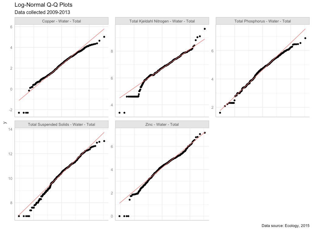
Figure 4.2 Quantile-quantile plots of COCs using a natural-log (ln) scale. Red line shows the QQ-line.
Spatial Data
For this study, we did not rely on the permittee’s self-reported land use type to run regression models predicting pollution loading from land use. A visual scan of our land cover data layer versus self-reported land use types revealed little agreement among permittee definitions of the four land use types (high density residential, low density residential, commercial, industrial). Therefore, we compiled a suite of continuous datasets from which to run chemical loading models. We divide these into land use and landscape data.
Land Use
In order to employ a consistent analysis across different monitored watersheds we extracted land use data from the Washington Department of
Commerce Land Use: Puget Sound Mapping Project.
Land use classes (also listed in Table 4.2) include:
-
Intensive urban (includes commercial areas, apartment buildings)
-
Urban residential (includes the majority of urban and suburban single-family dwellings)
-
Rural residential
-
Industrial
In addition, we combined some land use classes to generate additional land use classes:
-
Total residential (urban residential + rural residential)
-
Intensive Urban + Industrial; the industrial land use category did not have many non-zero data points
Landscape Data
For each watershed contained in the S8 dataset, potentially relevant landscape data were extracted from the following sources (Table 4.2):
Table 4.2: Sources of landscape spatial predictor data used to develop statistical models.
| Layer | ID | Source |
|---|---|---|
| urban residential | urbRES | Washington State Department of Commerce, Puget Sound Mapping Project |
| rural residential | ruRES | |
| total residential (urban + rural) | totRES | |
| intensive urban | intURB | |
| industrial | IND | |
| intensive urban + industrial | intURB_IND | |
| impervious surfaces | impervious | |
| paved surfaces | paved | |
| rooftop density | roofs | |
| urban residential rooftops | r oof_urbRES | rooftop density applied to Washington State Department of Commerce, Puget Sound Mapping Project data |
| total residential rooftops | r oof_totRES | |
| intensive urban rooftops | r oof_intURB | |
| intensive urban + industrial rooftops | roof_ intURB_IND | |
| grass & low vegetation | grass | |
| tree cover | trees | |
| total vegetative cover | greenery | |
| undeveloped areas | nodev | |
| traffic | traffic | |
| population | popn | |
| particulate matter 2.5um | pm25_na | |
| particulate surface area | partSA | |
| NO2 | no2 | |
| carbon emissions, commercial | CO2_com | Vulcan Carbon Dioxide Emissions data set |
| carbon emissions, residential | CO2_res | |
| carbon emissions, road | CO2_road | |
| carbon emissions, nonroad | C O2_nonroad | |
| carbon emissions, total | CO2_tot | |
| slope | slope | |
| age of development | devAge | Calculated value based on year of development |
Pre-processing of spatial data
In order to use the landscape data at an appropriate scale across the study area, spatial predictors were stacked and then convolved with a 100-meter gaussian kernel. This resulted in “fuzzy” predictors that could apply across dataset boundaries. These values were then extracted for each monitored watershed.
Prior to use, spatial data were plotted and visually assessed for outliers (Fig. 4.3). Square-root transformation was performed on spatial data sets with outliers that were higher than the rest of the predictor’s values: popn, traffic, slope, CO2_res, CO2_com, CO2_road, CO2_nonroad, CO2_tot. The devAge spatial predictor had a low data outlier; devAge values were squared to address the low outlier. Figure 4.4 shows the spatial data following transformation.
Prior to use in models, spatial data sets were scaled and centered using the mean and standard deviation from the 14 watersheds in this study.
![]()
Figure 4.3 Raw spatial data
![]()
Figure 4.4 Spatial data following transformation
Precipitation Data
Daily rainfall data were obtained from the DayMet website operated by NASA. Daily data were obtained for years
2009 to 2013, and cumulative one day, three day, and seven day, 14-day, 21-day and 28-day antecedent precipitation were calculated for each sampling date. For example, for a sampling date of March 22, cumulative three-day precipitation would include precipitation occurring on March 20, 21 and 22. For each COC, ln-transformed chemical concentrations were plotted against each precipitation measurement, and the plots were visually assessed to select the most appropriate time scale for precipitation. Cumulative 21-day precipitation was selected for copper and phosphorus, while 1-day precipitation was selected for TSS.
Model Construction and Selection
Selection of the best model for each COC was performed using the methodology of Zuur al. (2009), as outlined in the steps below. Statistical analyses and model fitting were performed in R (R Core Team, 2021).
Step 1. Select strong potential landscape predictors
The initial step was to find a suitable set of potential landscape predictors for the COC in question. Single-predictor linear models were constructed for the relationship between ln-transformed chemical concentration and each landscape predictor, in turn. Plots were visually assessed to determine candidate predictors for linear mixed effects models. We looked for slopes with a p-value of < 0.05, and for data points to fall roughly along the best fit model line. If prior knowledge indicated the importance of certain predictors, those were also included in the set of candidate predictors.
Step 2. Construct a beyond-optimal model, controlling for collinearity
The starting point of our model selection process was a “beyond-optimal” model, where the fixed component of the mixed effects model contained as many strong landscape predictors as possible. To prevent using highly correlated landscape predictors together in statistical models, we calculated calculated the correlation coefficient for each coefficient pair of landscape predictors, and eliminated select predictors to reduce correlation. We then constructed a generalized leas squared (gls) model in R (nlme package, Pinheiro et al., 2021) using the beyond-optimal set of fixed effects, and utilizing restricted maximum likelihood estimation (REML).
Throughout the model selection process, highly correlated landscape predictors (correlation coefficient ≥0.85) were not used together in any models.
Step 3. Control for heterogeneity (heteroskedasticity)
Normalized residuals from the “beyond-optimal” gls model were plotted against the model’s fitted values, and examined for heteroskedasticity. We also plotted residuals against agency, year, season, land use, precipitation, antecedent dry days, and all potential predictors, to look for patterns in residuals. If residual plots showed evidence of heteroskedasticity, we tried a series of gls models (fitted with REML) with different variance structures that utilized agency, season, and precipitation as variance covariates. Variance structure for each COC was selected based on the lowest Akaike information criterion (AIC) and Bayesian information criterion (BIC) scores.
Step 4. Find the proper random effects structure
Next, we used the beyond-optimal model with the correct variance structure to find the proper random effects structure. The beyond-optimal gls model was compared to a linear mixed effects (lme) -random intercept model (nlme package, Pinheiro et al., 2021) fitted with REML, where the intercept was allowed to change per agency. Because the gls model and the random intercept model are nested, the two models were compared using a likelihood ratio test to see if one model was significantly better than the other (p-value < 0.05). The best-fit model was then selected based on the lowest AIC value. For all COCs, the random intercept model fit the data better than the gls model with no random effects.
A random intercept for agency is suitable for the stormwater data because there were opportunities for each agency to differ slightly in sample collection methodologies. Selection of lab for sample analysis, timing of sample collection once a storm began, and any biases in selection of representative watersheds by each agency are possible factors that could lead to unintended differences in COC results. These unintended differences can be captured in the random component of the model.
Step 5. Check for temporal and spatial correlation
The beyond-optimal model with the correct variance structure and random effects structure was then examined for evidence of temporal and spatial auto-correlation. Temporal auto-correlation plots were generated and visually assessed for indications of correlation between various sampling time lags; no evidence of temporal autocorrelation was found for any COC.
To assess for spatial auto-correlation, we used two methods: variograms, and spatially-explicit bubble plots of model residuals.
All tests for temporal and spatial auto-correlation were repeated following selection of best-fit models.
Step 6. Find the proper fixed effects structure
We used the strong potential landscape predictors from step 1 to generate an exhaustive set of fixed-effects formulae with combinations of one, two and three potential landscape predictors. Predictors with high correlation coefficients (≥0.85) were not allowed to be in formulae together.
A set of models was generated using the fixed effects formulae, along with the best-fit random effects and variance structures identified in steps 3 and 4. Linear mixed effects models were applied using the nlme package (Pinheiro et al, 2021), and fitting with maximum likelhood (ML) estimation[2]. Models where the sign (+ or –) of the predictor coefficients did not match the coefficient signs from the linear model from step 1 were discarded. Models were then sorted according to AIC value, and the top 20 models were examined for fit to individual predictors. Plots of residuals versus fitted values, agency, location, and landscape predictors were also examined. Based on these criteria, one to three models were selected for consideration as the best landscape predictor model. The top one to three candidate models all had low AIC values, decent residual plots, and good fit to individual landscape predictors.
Using knowledge of chemical contaminant mobilization into stormwater, we selected the best landscape predictor model for each COC.
Final model comparison
Three models were ultimately fitted with REML and compared for each COC:
-
Null Model: COC concentration is equal to median COC concentration over all sampling dates and locations
-
Categorical Land Use Model: COC concentration is modeled as a linear mixed effects model, utilizing land use category (HDR, LDR, COM, IND), precipitation (rainfall and/or antecedent dry days), and season (for COCs where a seasonal trend appeared in the data).
-
Landscape Predictor Model: COC concentration is modeled as a linear mixed effects model, utilizing up to three landscape predictors, precipitation (rainfall and/or antecedent dry days), and season (for COCs where a seasonal trend appeared in the data).
Results
Results for each COC are provided below.
Copper
Based on linear models of ln-transformed copper versus individual predictors, the strong predictors identified for copper include: totRes, intURB, intURB_IND, grass, greenery, impervious, nodev, sqrt_traffic, sqrt_popn, pm25_na, sqrt_CO2_tot, sqrt_CO2_com, sqrt_CO2_road, sqrt_CO2_nonroad, devAge2, roof_intURB_IND (Fig 4.5).
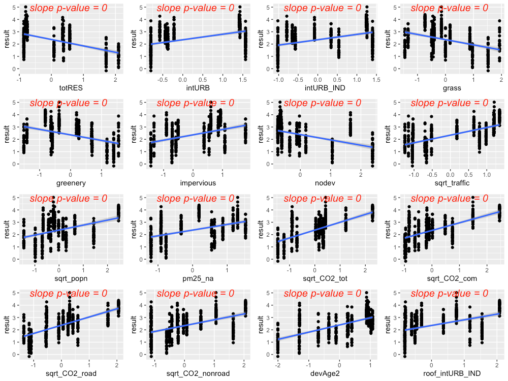
Figure 4.5 Strong predictors for copper, showing linear model fit (blue line) for the relationship between ln-transformed copper concentration and each predictor in turn.
The precipitation predictor used for copper was 21-day cumulative precipitation. In addition, evidence of higher copper concentrations during summer led us to add summer as a categorical predictor to the copper model (where summer = 1 during July, August, September, and summer = 0 for all other months).
Residuals plotted against fitted values showed signs of slight heterogeneity (Fig 4.6, left plot). Of the variance structures tested, the best fit allows residual variation to differ by agency j
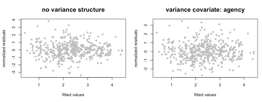
Figure 4.6 Normalized residuals from beyond-optimal model, with no variance structure (left), and with the best fit variance structure (right).
The best model for copper is a random-intercept model, where the intercept of the linear model is allowed to shift up or down according to agency. No signs of temporal or spatial auto-correlation were detected in auto-correlation plots or variograms.
With the variance structure and random components set, two possible models emerged to capture the fixed effects:
The first model’s AIC score was lower than that of the second model (AIC=756.3 vs. 781.8, when models were fitted with ML); however, the model coefficient for totRES is negative, indicating that increased residential zoning results in reduced copper concentrations in stormwater. This relationship makes sense for the 14 watersheds in our study, but would likely not be appropriate for forested landscapes that have low residential zoning (thus should have high copper concentrations). As a result, we selected the second model as the most suitable for covering the entire area of the stormwater heatmap. Figure 4.7 shows the model fit for each individual predictor, plotted against data points. Correlation between the three predictors was low (maximum correlation = 0.4). Figure 4.8 shows the interaction between rain and pm25_na, with higher pm25_na values in reds and oranges, and lower pm25_na values in blues and purples. This interaction shows that, when pm2.5 values are high, increasing amounts of rainfall result in a dilution of copper in stormwater.
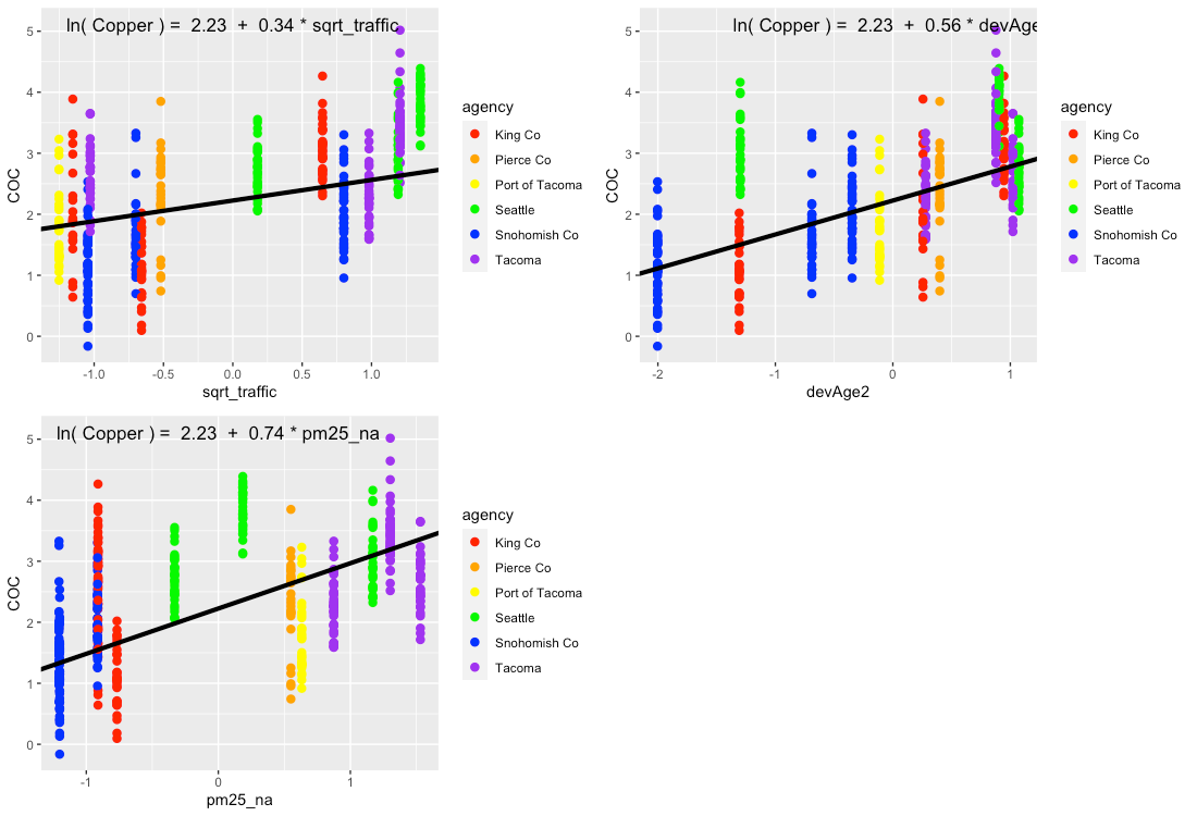
Figure 4.7 Single-predictor plots for copper, showing fit of the Landscape Predictor Model to each predictor in turn. Model fitting was performed using maximum likelihood (ML) estimation.
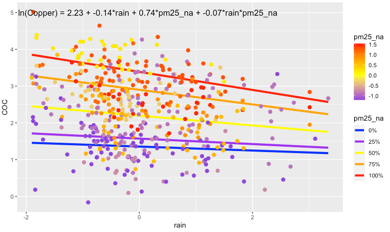
Figure 4.8 Plot showing the interaction between rain and pm25_na that is present in the best fit model. In areas with high pm25_na values, increasing amounts of rain result in a dilution of copper in stormwater. Model fitting was performed using maximum likelihood (ML) estimation.
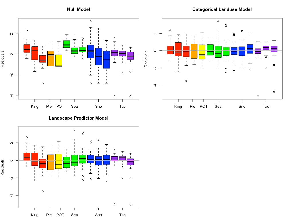
Comparisons between the Null Model, Categorical Land Use Model, and Landscape Predictor Model can be visualized through residuals (Fig. 4.9), comparative metrics such as AIC (Table 4.3, and coefficient values (Table 4.2; Fig. 4.10). Although the AIC value for the Categorical Land Use Model is lower than that of the Landscape Predictor Model, we are not confident in the transferability of the Categorical Land Use Model to watersheds outside of the 14 in this study. Two of the land use categories (Industrial – IND; and Low Density Residential – LDR) each have only two watershed representatives in our study. This results in good model fit to the data, but not necessarily for all watersheds in Puget Sound area.
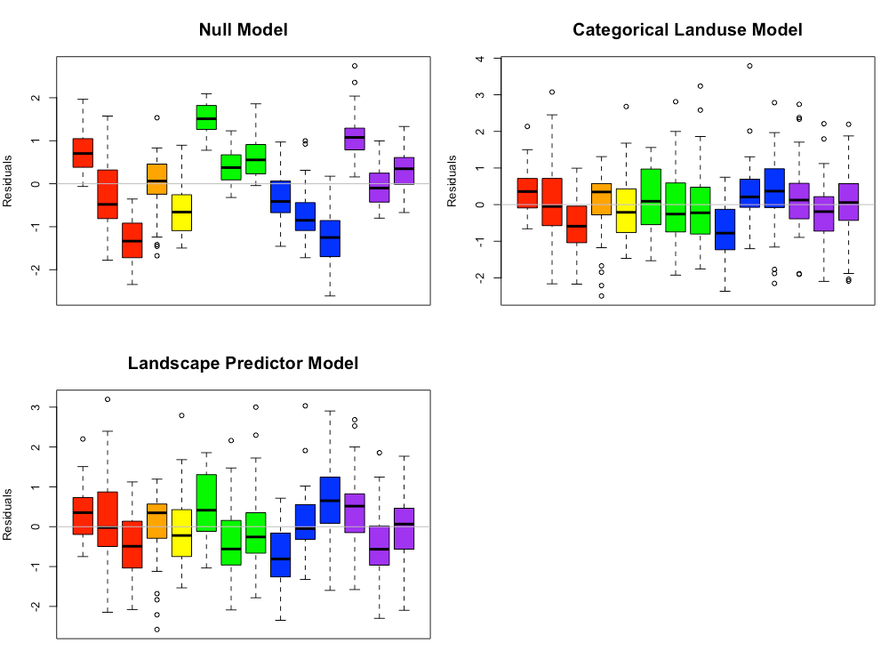
Figure 4.9 Copper model residuals for the Null Model, Categorical Land Use Model, and Landscape Predictor Models. Each bar represents one watershed, with colors representing agencies. Model fitting was performed using maximum likelihood (ML) estimation.
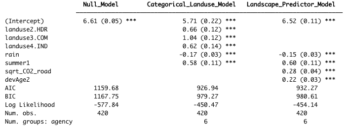
Table 4.3 Coefficient values (standard error in parenthesis) for the three copper models. For the Categorical Landuse Model, the baseline landuse is LDR; all other land use categories are adjustments from the baseline. Final coefficient values for linear mixed effects mdels are based on fitting with restricted maximum likelihood (REML) estimation, and may differ slightly from those fitted using maximum likelihood (ML) estimation.
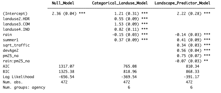
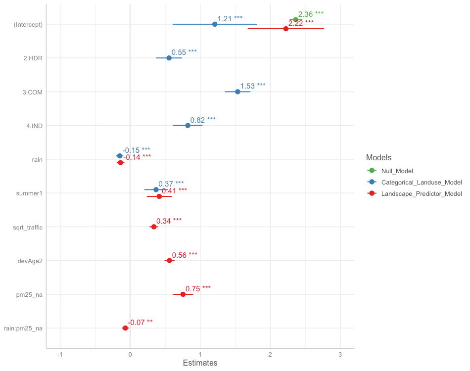
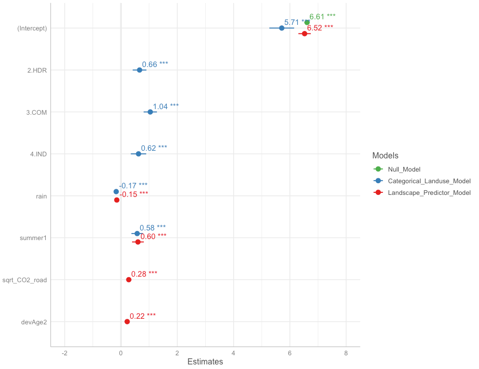
Figure 4.10 Model coefficients for the Null Model (green), Categorical Land Use Model (blue), and Landscape Predictor Model (red). Final coefficient values for linear mixed effects models are based on fitting with restricted maximum likelihood (REML) estimation, and may differ slightly from those fitted using maximum likelihood (ML) estimation.
The Landscape Predictor Model for total copper, used as the basis for the Stormwater Heatmap total copper layer, is:
where rain is 21-day cumulative precipitation, and summer is a factor with value = 1 for July, August, September, and value = 0 for all other months. Note that all predictors (except summer) were first transformed if necessary (e.g. traffic was square-root transformed, devAge was squared to make devAge2), then standardized prior to use.
Total Suspended Solids
Based on linear models of ln-transformed TSS versus individual predictors, the strong predictors identified for TSS include: totRES, sqrt_traffic, sqrt_popn, sqrt_CO2_res, sqrt_CO2_tot, sqrt_CO2_com, sqrt_CO2_road, devAge2 (Fig 4.11). Paved was added to the list because it was a strong predictor for an older version of the model, and paved areas are associated with elevated TSS in stormwater.
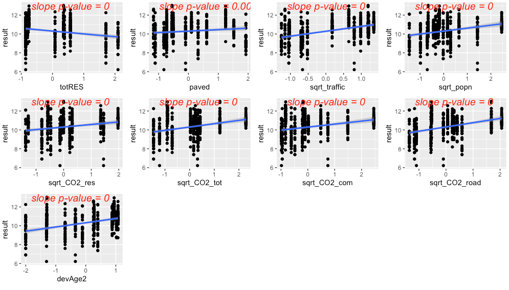
Figure 4.11 Strong predictors for TSS, showing linear model fit (blue line) for the relationship between ln-transformed TSS concentration and each predictor in turn. Although it wasn’t as compelling on its own, the predictor paved was added to the list of strong predictors because it was a strong predictor in a previous model.
The precipitation predictor used for TSS was 1-day cumulative precipitation. There was no evidence of seasonal patterns to TSS in stormwater.
Residuals plotted against fitted values showed signs of slight heterogeneity (Fig 4.12, top left plot). Of the variance structures tested, the best fit was for a combination of two variance structures, where residual variation differs by agency j, and also by rainfall at each location i and date k: Residuals plotted against fitted values showed signs of slight heterogeneity (Fig 4.12, top left plot). Of the variance structures tested, the best fit was for a combination of two variance structures, where residual variation differs by agency j, and also by rainfall at each location i and date k:
The second best fit allows residual variation to differ by agency j:
Visual inspection of residuals generated using the two candidate variance structures did not indicate a strong benefit to using the more complex variance structure. As a result, we used the simpler variance structure with only agency as a variance covariate.
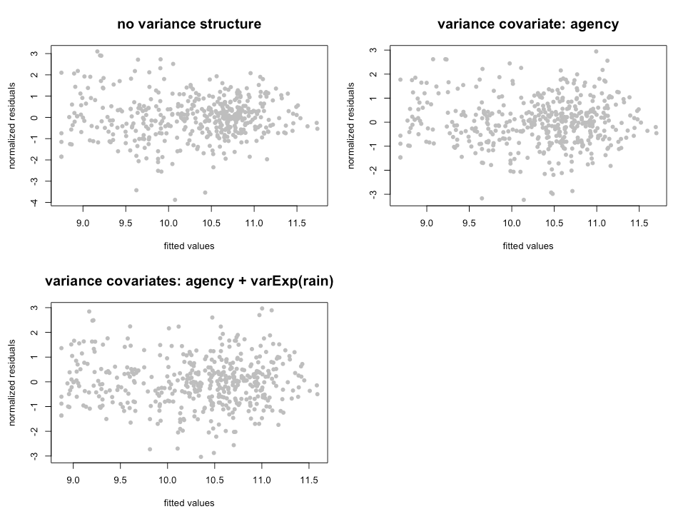
Figure 4.12 Normalized residuals from beyond-optimal model, with no variance structure (top left), agency as a variance covariate (top right) and the best fit variance structure with agency and rain as variance covariates (bottom left).
The best model for TSS is a random-intercept model, where the intercept of the linear model is allowed to shift up or down according to agency. No signs of temporal or spatial auto-correlation were detected in auto-correlation plots or variograms.
With the variance structure and random components set, two possible models emerged to capture the fixed effects:
The AIC score for these two models was very close, with the first model’s AIC score slightly lower (AIC=1253.5 vs. 1255.8, when models were fitted with ML). In the first model, the coefficient for totRES is negative, indicating that increased residential zoning results in reduced TSS in stormwater. This relationship makes sense for the 14 watersheds in our study, but would likely not be appropriate for forested landscapes that have low residential zoning (thus should have high TSS concentrations). As a result, we selected the second model as the most suitable for covering the entire area of the stormwater heatmap. Figure 4.13 shows the model fit for each individual predictor, plotted against data points. Correlation between the two predictors was low (correlation coefficient < 0.1).
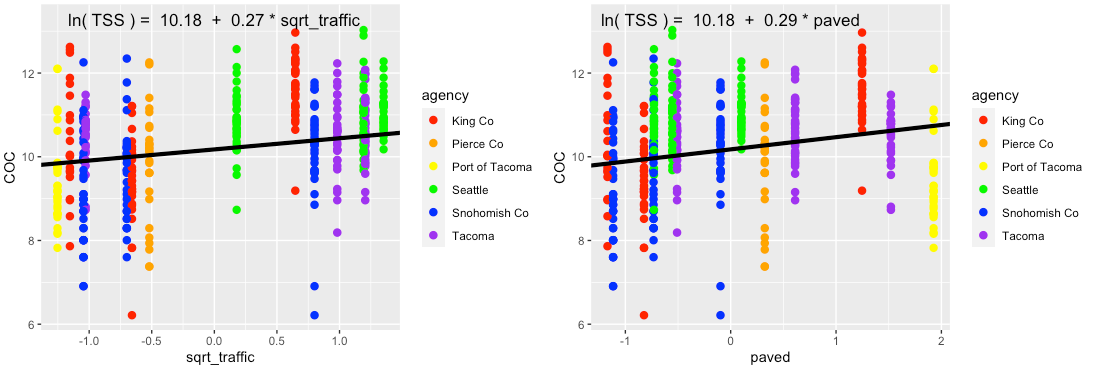
Figure 4.13 Single-predictor plots for TSS, showing fit of the Landscape Predictor Model to each predictor. Model fitting was performed using maximum likelihood (ML) estimation.
Comparisons between the Null Model, Categorical Land Use Model, and Landscape Predictor Model can be visualized through residuals (Fig. 4.14) comparative metrics such as AIC and BIC (Table 4.4), and coefficient values (Table 4.4; Fig. 4.15). The AIC value is slightly lower for the Categorical Landuse Model than for the Landscape Predictor Model, but the BIC metric is opposite, with the Landscape Predictor Model indicated as the best model. While the two models may have similar statistical test metrics, we are not confident in the transferability of the Categorical Landuse Model to watersheds outside of the 14 in this study. Two of the land use categories (Industrial - IND; and Low Density Residential - LDR) each have only two watershed representatives in our study, resulting in good model fit to the data, but not necessarily for all watersheds in Puget Sound area.
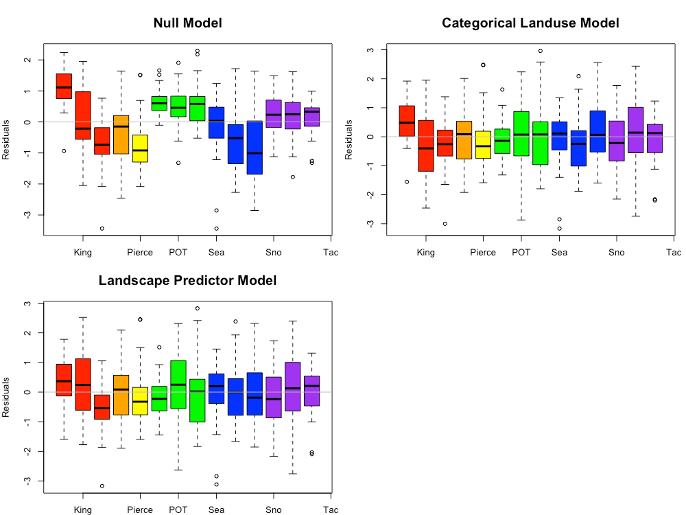
Figure 4.14 TSS model residuals for the Null Model, Categorical Land Use Model, and Landscape Predictor Models. Each bar represents one watershed, with colors representing agencies.
Table 4.4 Coefficient values (standard error in parenthesis) for the three TSS models. For the Categorical Landuse Model, the baseline landuse is LDR; all other land use categories are adjustments from the baseline. Final coefficient values for linear mixed effects. Final coefficient values for linear mixed effects models are based on fitting with restricted maximum likelihood (REML) estimation, and may differ slightly from those fitted using maximum likelihood (ML) estimation.
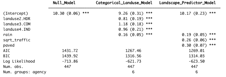
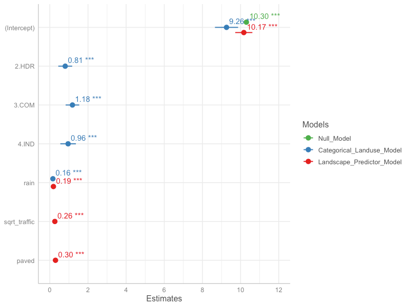
Figure 4.15 Model coefficients for the Null Model (green), Categorical Land Use Model (blue), and Landscape Predictor Model (red).Final coefficient values for linear mixed effects models are based on fitting with restricted maximum likelihood (REML) estimation, and may differ slightly from those fitted using maximum likelihood (ML) estimation.
The final Landscale Predictor Model for TSS, used as the basis of the Stormwater heatmap TSS layer, is:
where rain is 1-day cumulative precipitation. Note that all predictors were standardized prior to use.
Phosphorus
Based on linear models of ln-transformed phosphorus versus individual predictors, the strong predictors identified for phosphorus include: sqrt_traffic, sqrt_popn, sqrt_slope, sqrt_CO2_res, sqrt_CO2_tot, sqrt_CO2_road and devAge2 (Fig 4.16). Paved and grass were added to the list because they were strong predictors for an older version of the model, and both are associated with elevated phosphorus in stormwater.
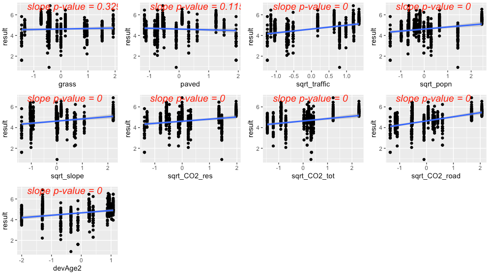
Figure 4.16 Strong predictors for phosphorus, showing linear model fit (blue line) for the relationship between ln-transformed phosphorus concentration and each predictor in turn. Although they weren’t compelling on their own, the predictors grass and paved were added to the list of strong predictors because they were strong predictors in a previous model.
The precipitation predictor used for phosphorus was 21-day cumulative precipitation. In addition, evidence of higher phosphorus concentrations during summer led us to add summer as a categorical predictor to the phosphorus model (where summer = 1 during July, August, September, and summer = 0 for all other months).
Residuals plotted against fitted values showed signs of slight heterogeneity (Fig 4.17, left plot). Of the variance structures tested, the best fit allows residual variation to differ by agency j:
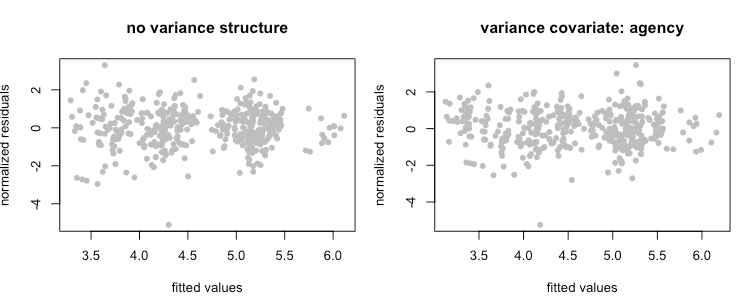
Figure 4.17 Normalized residuals from beyond-optimal model, with no variance structure (left), and with the best fit variance structure (right).
The best model for phosphorus is a random-intercept model, where the intercept of the linear model is allowed to shift up or down according to agency. No signs of temporal or spatial auto-correlation were detected in auto-correlation plots or variograms.
With the variance structure and random components set, two possible models emerged to capture the fixed effects:
The AIC score for these two models was close, with the first model’s AIC score lower than that of the second model (AIC=830.3 vs. 839.8, when models were fitted with ML). As a result, we selected the first model. Figure 4.18 shows the model fit for each individual predictor, plotted against data points. Correlation between grass and paved was relatively high (-0.8), while the other correlation coefficients were lower (-0.4, -0.1). While this model fit the 14 watersheds in our study, the high negative correlation betweeen paved and grass indicates the need for caution with this model. There is good evidence to support a positive relationship between phosphorous concentration and both residential lawns (fertilizer) and paved roadways. For example, Waschbusch et al. (1999) found that lawns and roads contributed ~80% of total and dissolved phosphorous loading. Land use affects the contribution from different sources, with lawns and leaf litter being more important in residential areas and roads being more important in commercial and industrial areas.
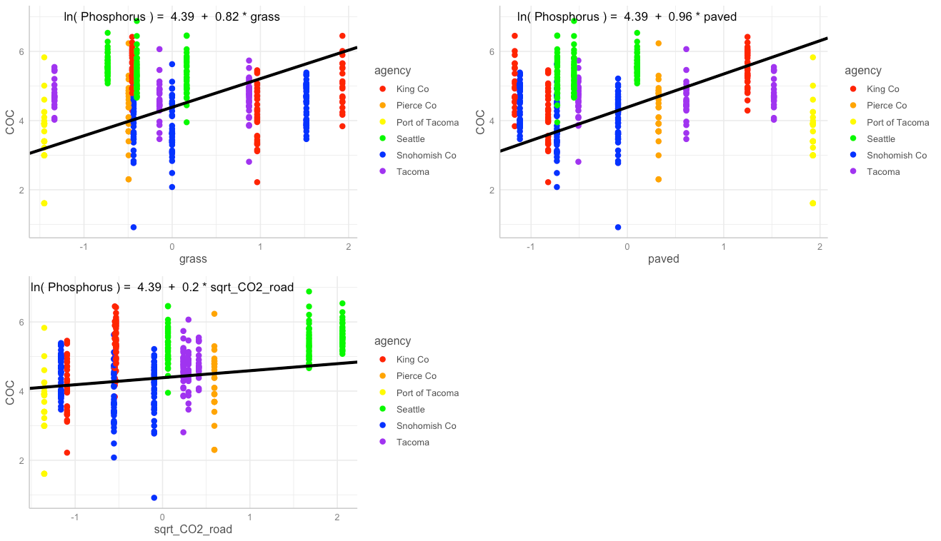
Figure 4.18 Single-predictor plots for phosphorus, showing fit of the Landscape Predictor Model to each predictor. Model fitting was performed using maximum likelihood (ML) estimation.
Comparisons between the Null Model, Categorical Land Use Model, and Landscape Predictor Model can be visualized through residuals (Fig. 4.19), comparative metrics such as AIC (Table 4.5), and coefficient values (Table 4.5; Fig. 4.20). The lowest AIC value is for the Landscape Predictor Model, indicating best fit to the phosphorus data of these three models.
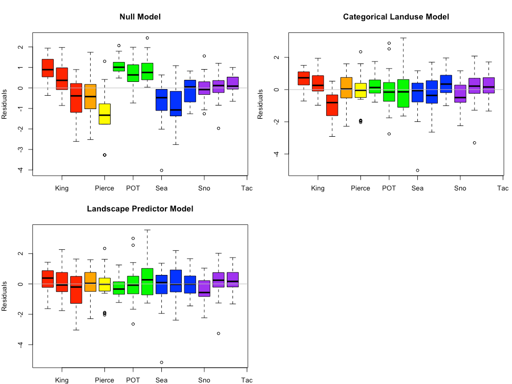
Figure 4.19 Phosphorus model residuals for the Null Model, Categorical Land Use Model, and Landscape Predictor Models. Each bar represents one watershed, with colors representing agencies. Model fitting was performed using maximum likelihood (ML) estimation.
Table 4.5 Coefficient values (standard error in parenthesis) for the three phosphorus models. For the Categorical Landuse Model, the baseline landuse is LDR; all other land use categories are adjustments from the baseline. Final coefficient values for linear mixed effects models are based on fitting with restricted maximum likelihood (REML) estimation, and may differ slightly from those fitted using maximum likelihood (ML) estimation.
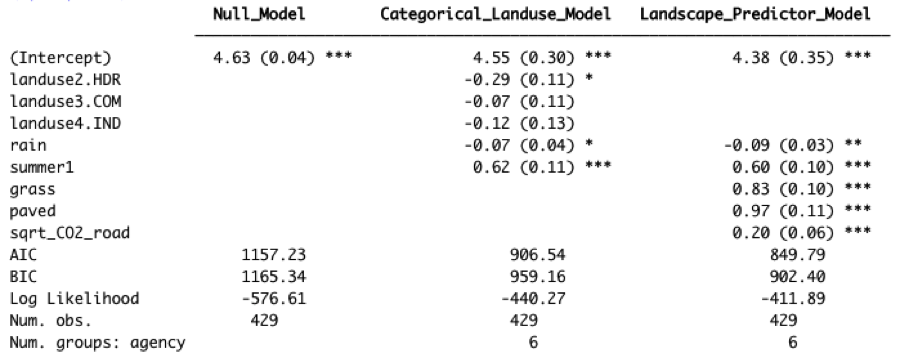
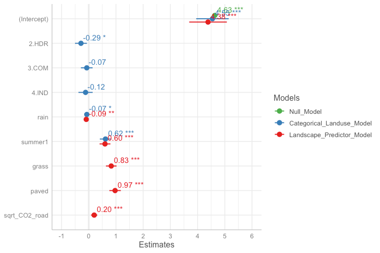
Figure 4.20 Model coefficients for the Null Model (green), Categorical Land Use Model (blue), and Landscape Predictor Model (red). Final coefficient values for linear mixed effects models are based on fitting with restricted maximum likelihood (REML) estimation, and may differ slightly from those fitted using maximum likelihood (ML) estimation.
The Landscape Predictor Model for phosphorous, used as the basis for the Stormwater Heatmap phosphorous layer, is:
where rain is 21-day cumulative precipitation, and summer is a factor with value = 1 for July, August, and September, and value = 0 for all other months. Note that all predictors (except summer) were first transformed if necessary (the square root was taken of CO2_road to generate sqrt_CO2_road), then standardized prior to use.
Total Zinc
Based on linear models of ln-transformed total zinc versus individual predictors, the strong predictors identified for total zinc include: totRES, intURB_IND, grass, greenery, paved, impervious, trees, sqrt_traffic, pm25_na, sqrt_CO2_tot, sqrt_CO2_com, sqrt_CO2_nonroad, roof_intURB_IND (Fig 4.21).
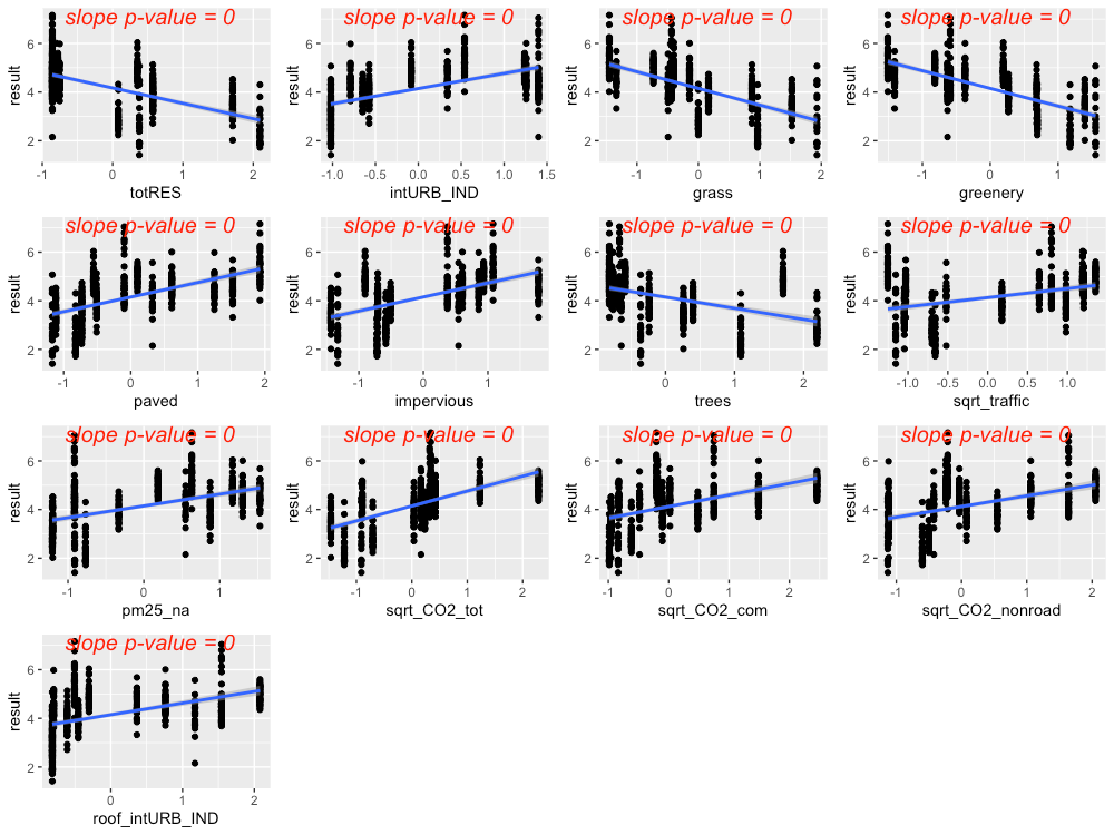
Figure 4.21 Strong predictors for total zinc, showing linear model fit (blue line) for the relationsihp between ln-transformed total zince concentration and each predictor in turn.
The precipitation predictor used for total zinc was 14-day cumulative precipitation. In addition, evidence of higher total zinc concentrations during summer led us to add summer as a categorical predictor to the total zinc model (where summer = 1 during July, August, and September, and summer= 0 for all other months).
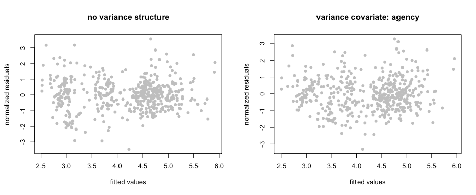
Residuals plotted against fitted values showed a pattern, indicating a chance of slight heteroskedasticity (Fig. 4.22, left plot). Of the variance structures tested, the best fit allows residual variation to differ by agency j.
 Figure
4.22 Normalized residuals from beyond-optimal model, with no variance
structure (left), and with the best fit variance structure (right).
Figure
4.22 Normalized residuals from beyond-optimal model, with no variance
structure (left), and with the best fit variance structure (right).
The best model for total zinc is a random-intercept model, where the intercept of the linear model is allowed to shift up or down according to agency. No signs of temporal or spatial auto-correlation were detected in auto-correlation plots or variograms.
With the variance structure and random components set, three possible models emerged to capture the fixed effects:
The AIC scores for these three models were close, with the first model’s AIC score lower than that of the second or third models (AIC=784.6 vs. 788.1 and 792.1, when models were fitted with ML). As a result, we selected the first model. Figure 4.23 shows the model fit for each individual predictor, plotted against data points. Correlation between the three predictors was low (maximum correlation coefficient = 0.5). Figure 4.24 shows the interaction between rain and pm25_na, with higher pm25_na values in reds and oranges, and lower pm25_na values in blues and purples. This interaction shows that, when pm2.5 values are high, increasing amounts of rainfall result in a dilution of zinc in stormwater.
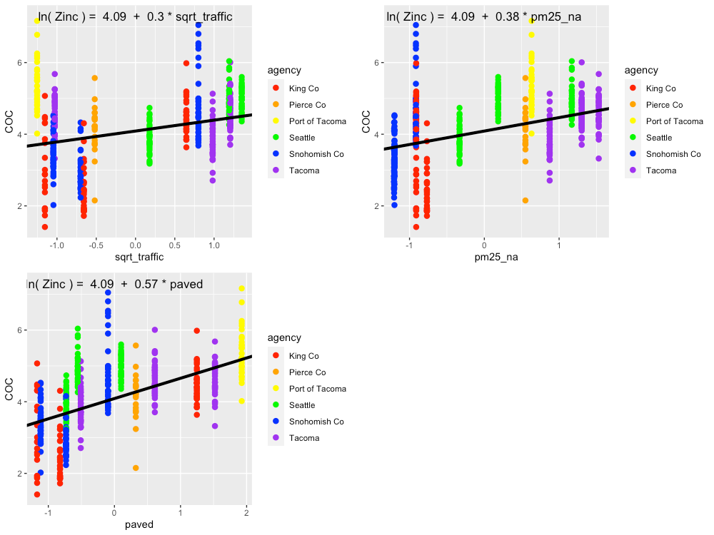
Figure 4.23 Single-predictor plots for total zinc, showing fit of the Landscape Predictor Model to each predictor. Model fitting was performed using maximum likelihood (ML) estimation.
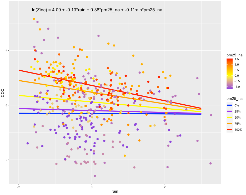
Figure 4.24 Plot showing the interaction between rain and pm25_na that is present in the best fit model. In areas with high pm25_na values, increasing amounts of rain result in a dilution of copper in stormwater. Model fitting was performed using maximum likelihood (ML) estimation.
Comparisons between the Null Model, Categorical Land Use Model, and Landscape Predictor Model can be visualized through residuals (Fig. 4.25) and also coefficient values (Table 4.6; Fig. 4.26). The lowest AIC value is for the Landscape Predictor Model, indicating best fit to the total zinc data of these three models.
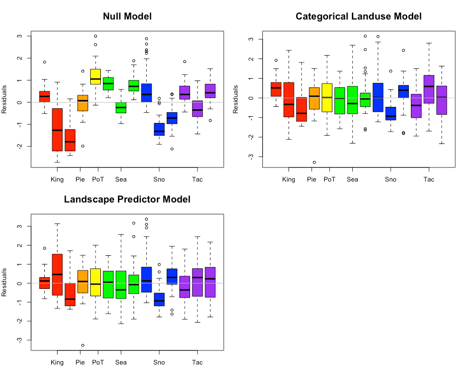 Figure
4.25 Total zinc model residuals for the Null Model, Categorical Land
Use Model, and Landscape Predictor Models. Each bar represents one
watershed, with colors representing agencies. Model fitting was
performed using maximum likelihood (ML) estimation.
Figure
4.25 Total zinc model residuals for the Null Model, Categorical Land
Use Model, and Landscape Predictor Models. Each bar represents one
watershed, with colors representing agencies. Model fitting was
performed using maximum likelihood (ML) estimation.
Table 4.6 Coefficient values (standard error in parenthesis) for the three total zinc models. For the Categorical Landuse Model, the baseline landuse is LDR; all other land use categories are adjustments from the baseline. Final coefficient values for linear mixed effects models are based on fitting with REML, and may differ slightly from coefficient values based on fitting with ML.
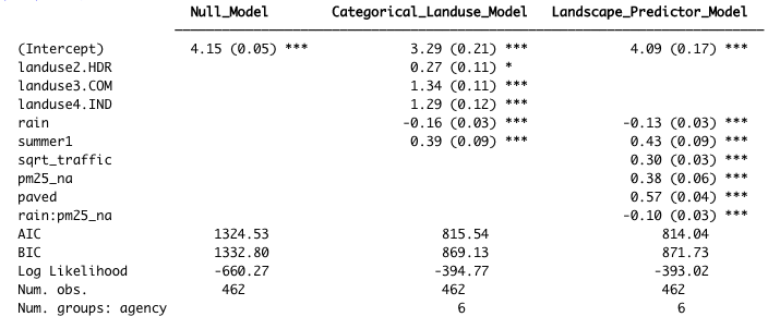
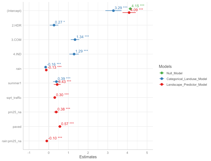 Figure 4.26 Model
coefficients for the Null Model (green), Categorical Land Use Model
(blue), and Landscape Predictor Model (red). Final coefficient values
for linear mixed effects models are based on fitting with REML, and may
differ slightly from coefficient values based on fitting with ML.
Figure 4.26 Model
coefficients for the Null Model (green), Categorical Land Use Model
(blue), and Landscape Predictor Model (red). Final coefficient values
for linear mixed effects models are based on fitting with REML, and may
differ slightly from coefficient values based on fitting with ML.
The landscape predictor model for total zinc, used as the basis for the Stormwater Heat Map total zinc layer, is:
where rain is 14-day cumulative precipitation, and summer is a factor with value=1 for July, August, September, and value=0 for all other months. Note that all predictors (except summer) were were first transformed if necessary (the square root was taken of traffic to generate sqrt_traffic), then standardized prior to use.
Total Kjeldahl Nitrogen
Out of 420 Total Kjeldahl nitrogen (TKN) samples, 41 samples (9.8%) were flagged as non-detects, with a variety of detection limits ranging from 30 to 500. The majority of non-detect samples came from three agencies: Pierce County, Port of Tacoma, and Snohomish County (Fig. 4.27). High detection limits in Pierce County and Port of Tacoma strongly truncated the lower half of these data sets.
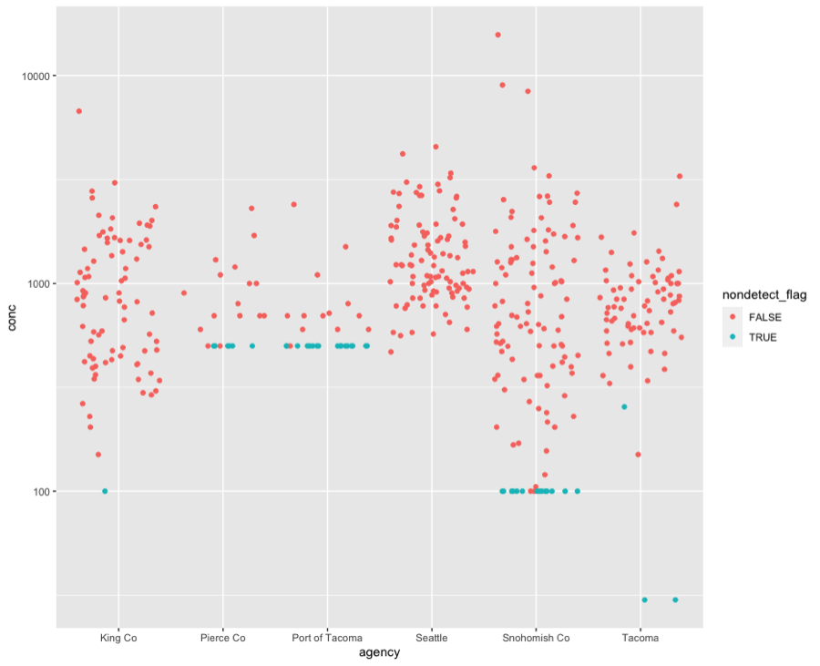 Figure 4.27
Concentrations of total Kjeldahl nitrogen in samples collected by
agency. Red dots indicate detected values, while blue dots indicate the
detection limit for samples flagged as non-detect.
Figure 4.27
Concentrations of total Kjeldahl nitrogen in samples collected by
agency. Red dots indicate detected values, while blue dots indicate the
detection limit for samples flagged as non-detect.
Based on linear models of ln-transformed TKN versus individual predictors, the strong predictors identified for TKN include: roofs, nodev, traffic, sqrt_popn, sqrt_CO2_res, sqrt_CO2_tot, sqrt_CO2_road, devAge2, roof_inURB and roof_intURB_IND (Fig. 4.28).
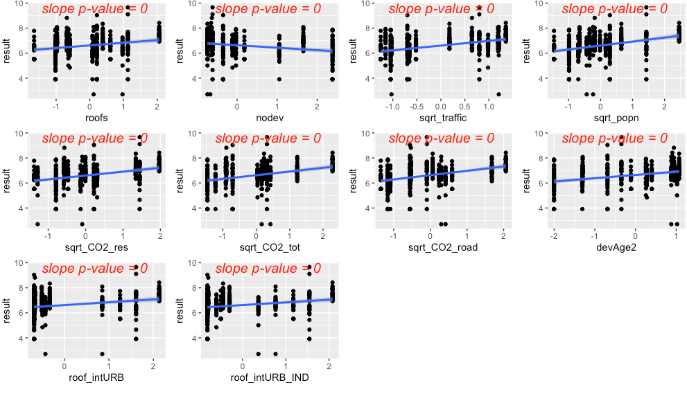 Figure
4.28 Strong predictors for total Kjeldahl nitrogen (TKN), showing
linear model fit (blue line) for the relationship between
ln-transformed TKN concentration and each predictor in turn.
Figure
4.28 Strong predictors for total Kjeldahl nitrogen (TKN), showing
linear model fit (blue line) for the relationship between
ln-transformed TKN concentration and each predictor in turn.
The precipitation predictor used for TKN was 14-day cumulative precipitation. In addition, evidence of higher TKN concentrations during summer led us to add summer as a categorical predictor to the TKN model (where summer = 1 during July, August, September, and summer = 0 for all other months).
Residuals plotted against fitted values showed signs of slight heterogeneity (Fig. 4.29, left plot). Of the variance structures tested, the best fit allows residual variation to differ by agency j.
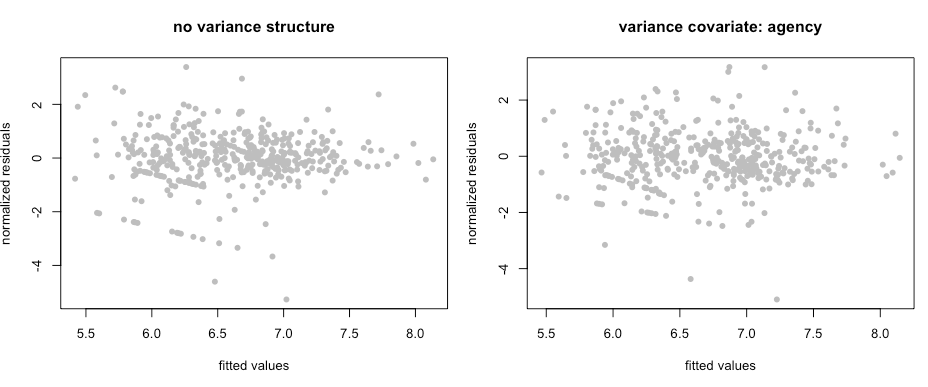 Figure
4.29 Normalized residuals from beyond-optimal model, with no variance
structure (left), and with the best fit variance structure (right).
Figure
4.29 Normalized residuals from beyond-optimal model, with no variance
structure (left), and with the best fit variance structure (right).
The best model for TKN is a random-intercept model, where the intercept of the linear model is allowed to shift up or down according to agency. No signs of temporal or spatial auto-correlation were detected in auto-correlation plots or variograms. With the variance structure and random components set, three possible models emerged to capture the fixed effects:
Each of these models captures two major contributors to total nitrogen: vehicles and amount/age of development. The AIC scores for all three models were close, with the models ordered from lowest to highest AIC score (907.8, 912.2, 915.8, when models were fitted using ML).
We selected the second model, with landscape predictors sqrt_CO2_road + devAge2. While all models fit the data reasonably well, we opted to use the slightly coarser-scale predictor sqrt_CO2_road rather than sqrt_traffic. The amount of traffic on Puget Sound freeways exceeds the traffic in our dataset by an order of magnitude, and the TKN vs. sqrt_traffic relationship may lose its linear shape at high traffic levels. In contrast, the CO2_road values in our dataset range from about 150 to 7900, while the range of pixel values for the entire Puget Sound region is 0 to 12,700. Less than 0.3% of pixels exceed 7900. This lends greater confidence to the TKN model with sqrt_CO2_road as a predictor. Figure 4.30 shows the model fit for each individual predictor, plotted against data points. Correlation between the two predictors was low (correlation coefficient = 0.4).
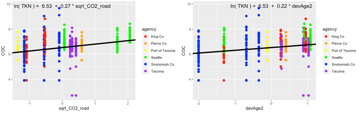 Figure 4.30
Single-predictor plots for total Kjeldahl nitrogen, showing fit of the
Landscape Predictor Model to each predictor. Model fitting was performed
using maximum likelihood (ML) estimation.
Figure 4.30
Single-predictor plots for total Kjeldahl nitrogen, showing fit of the
Landscape Predictor Model to each predictor. Model fitting was performed
using maximum likelihood (ML) estimation.
Comparisons between the Null Model, Categorical Land Use Model, and Landscape Predictor Model can be visualized through residuals (Fig. 4.31), comparative metrics such as AIC (Table 4.7), and coefficient values (Table 4.7; Fig. 4.32). Although the AIC value for the Categorical Land Use Model is lower than that of the Landscape Predictor Model, we are not confident in the transferability of the Categorical Land Use Model to watersheds outside of the 14 in this study. Two of the land use categories (Industrial – IND; and Low Density Residential – LDR) each have only two watershed representatives in our study. This results in good model fit to the data, but not necessarily for all watersheds in Puget Sound area.
 Figure
4.31 Total Kjeldahl nitrogen model residuals for the Null Model,
Categorical Land Use Model, and Landscape Predictor Models. Each bar
represents one watershed, with colors representing agencies. Model
fitting was performed using maximum likelihood (ML) estimation.
Figure
4.31 Total Kjeldahl nitrogen model residuals for the Null Model,
Categorical Land Use Model, and Landscape Predictor Models. Each bar
represents one watershed, with colors representing agencies. Model
fitting was performed using maximum likelihood (ML) estimation.
Table 4.7 Coefficient values (standard error in parenthesis) for the three total Kjeldahl nitrogen models. For the Categorical Landuse Model, the baseline landuse is LDR; all other land use categories are adjustments from the baseline. Final coefficient values for linear mixed effects models are based on fitting with restricted maximum likelihood (REML) estimation, and may differ slightly from those fitted using maximum likelihood (ML) estimation.
 Figure
4.32 Model coefficients for the Null Model (green), Categorical Land
Use Model (blue), and Landscape Predictor Model (red). Final coefficient
values for linear mixed effects models are based on fitting with
restricted maximum likelihood (REML) estimation, and may differ slightly
from those fitted using maximum likelihood (ML) estimation.
Figure
4.32 Model coefficients for the Null Model (green), Categorical Land
Use Model (blue), and Landscape Predictor Model (red). Final coefficient
values for linear mixed effects models are based on fitting with
restricted maximum likelihood (REML) estimation, and may differ slightly
from those fitted using maximum likelihood (ML) estimation.
Censored data made up 9.7% of the TKN sample results. Although the EPA allows substitution of (0.5 x detection limit) for censored values when < 15% of samples are non-detect (USEPA, 2009), we wanted to verify that substitution did not have a large effect on the parameter values for our dataset. Censored methods have not yet been developed for mixed effects models; as a result, we performed the (0.5 x detection limit) substitution for the TKN data, and fit a simple linear model using the predictors: 14-day rainfall, summer, sqrt_CO2_road and devAge2. We compared the parameter values to a censored data model using the NADA package in R (Lee, 2020), and found that the two models had very similar parameter values (Table 4.8). This confirmed that the TKN data with (0.5 x detection limit) substitution could be used to generate valid models using mixed effects techniques.
Table 4.8 Comparison of parameter values (standard error in parenthesis) generated by simplified linear models using two different methods to account for censored values.
| non-detects replaced with (0.5 * detection limit) | censored model | |
|---|---|---|
| (Intercept) | 6.57 (0.04) | 6.60 (0.04) |
| rain (14-day std) | -0.16 (0.04) | -0.16 (0.04) |
| summer | 0.67 (0.14) | 0.65 (0.13) |
| sqrt_CO2_road | 0.25 (0.04) | 0.24 (0.04) |
| devAge2 | 0.22 (0.04) | 0.21 (0.04) |
The Landscape Predictor Model for TKN, used as the basis for the Stormwater Heat Map TKN layer, is:
where rain is 14-day cumulative precipitation, and summer is a factor with value=1 for July, August, September, and value=0 for all other months. Note that all predictors (except summer) were first transformed if necessary (the square root was taken of CO2_road to generate sqrt_CO2_road; devAge was squared to generate devAge2), then standardized prior to use.
Translating Equations to the Stormwater Heatmap
The process of translating statistical equations for chemical contaminants to the Stormwater heatmap involved manipulation of the grid and equations.
Convolving the Base Map
The first step of translating COC equations to the Stormwater Heatmap was to convolve each grid on the base map. Following convolution of the map, regression equations were applied to each grid box to predict the concentration of contaminants expected for that grid box.
For COCs with traffic as a predictor (copper, TSS, zinc), the maximum traffic level in the grid map was clamped to 31,000 AADT. This upper limit corresponds to the maximum level of traffic found in the watersheds that provided data used for generating statistical equations. On freeways, which were not analyzed in this study, traffic conventrations can reach 240,000 AADT. By clamping traffic, we avoid extrapolating beyond the range of our data. This is a conservative approach because landscape predictors may not behave in a linear fashion at values beyond our range. Indeed, when the traffic level is clamped at 31,000 AADT for TSS, predicted TSS values on freeways are in the same range as those found on freeways across the country (data from USGS Highway Runoff Database). This suggests that, for some COCs, traffic may be a linear predictor over the values found in our data, but may reach an asymptote at higher values.
Applying Mixed Effects Equations to the Stormwater Heatmap
Utilizing a mixed effects model structure, along with a variance structure to account for heteroskedasticity, allowed us to obtain the best parameter values for each COC. The difference in parameter values generated by equations with and without random effects and/or variance structure illustrates how parameter values change according to the equation structure. For example, for total Kjeldahl nitrogen (TKN), regression values for each parameter can be compared for four models: 1) full model with random effects and variance structure, 2) random effects only (no variance structure), 3) variance structure only (no random effects), and 4) no random effects and no variance structure (Table 4.9). By specifying the correct random effects (i.e. random effects by agency) and variance structure (i.e. variance co-variate = agency) for TKN, we find the most appropriate fit to the data for the relationship between this COC and the suite of predictors.
With respect to translating mixed effects model equations to the Stormwater Heatmap to generate predictions for each grid box, the model becomes simplified. This is because we are interested in predicted COC values for the entire Puget Sound region, rather than the COC values that would be generated by the collection timing, analysis protocol, or biases of a specific agency. As such, we can largely ignore the agency-specific intercepts. We thus utilize the fitted value of the intercept for all watersheds and agencies in the Stormwater Heatmap, and do not adjust the intercept up or down according to agency. This allows us to predict COC values for the entire Puget Sound model domain, which is comprehensive of watersheds outside the agency boundaries for which we have monitoring data.
When it comes applying the variance structure to the full model domain of the heatmap, these effects have already been incorporated into the best fit model (Table 4.8). We accounted for the mild heteroskedasticity evident in COCs by specifying the variance structure to properly weigh the impact of each data point on the best fit model. No further extension of the variable structure is necessary for generating model predictions on the Stormwater Heatmap.
Table 4.9 Parameter values for four models of total Kjeldahl nitorgen: 1) full model with random effects and variance structure; 2)random effects only (no variance structure); 3) variance structure only (no random effects); 4) no random effects, no variance structure. Models are for illustrative purposes only, to show the effect of variance stucture and random effects on parameter values for predictor variables.
| Full Model | Random effects only | Variance structure only | |
|---|---|---|---|
| intercept | 6.523 | 6.521 | 6.642 |
| rain | -0.149 | -0.157 | -0.148 |
| summer | 0.603 | 0.675 | 0.606 |
| sqrt CO2 road | 0.276 | 0.276 | 0.277 |
| devAge2 | 0.220 | 0.240 | 0.203 |
Citations:
Faraway, Julian J, 2006. Extending the Linear Model with R: Generalized Linear, Mixed Effects and Nonparametric Regression Models. Boca Raton (FL): Chapman & Hall/CRC
Hobbs, W., B. Lubliner, N. Kale, and E. Newell, 2015. Western Washington NPDES Phase 1 Stormwater Permit: Final Data Characterization 2009-2013. Washington State Department of Ecology, Olympia, WA. Publication No. 15-03-001.
Lee, Lopaka, 2020. NADA: Nondetects and Data Analysis for Environmental Data. R package version 1.6-1.1.
Pinheiro J, Bates D, DebRoy S, Sarkar D, R Core Team, 2021. nlme: Linear and Nonlinear Mixed Effects Models. R package version 3.1-152.
R Core Team, 2021. R: A language and environment for statistical computing. R Foundation for Statistical Computing, Vienna, Austria.
U.S. Environmental Protection Agency, 2009, Statistical analysis of groundwater monitoring data at RCRA facilities, Unified guidance, EPA 530-R-09-007.
USGS Highway Runoff DataBase. Website visited 11/01/2021.
Waschbusch, R.J., W.R. Selbig, and R.T. Bannerman, 1999. Sources of Phosphorus in Stormwater and Street Dirt from Two Urban Residential Basins In Madison, Wisconsin, 1994–95. U.S. Geological Survey Water-Resources Investigations Report 99–4021.
Zuur AF, Ieno EN, Walker NJ, Saveliev AA, Smith GM. 2009. Mixed Effects Models and Extensions in Ecology with R. New York (NY): Springer
[1] Phase I Permittees include: cities of Tacoma and Seattle; King, Snohomish, Pierce and Clark counties; Ports of Tacoma and Seattle. For this study, all data were used with the exception of those from Clark County (outside of the Puget Sound region) and Port of Seattle (too different from all other Puget Sound watersheds).
[2] As described in Faraway (2006), pg 156, REML estimation should not be used to compare models with different fixed effects because REML estimates the random effects by considering linear combinations of the data that remove the fixed effects. If the fixed effects change, the likelihoods of the two models will not be directly comparable. However, REML is generally considered to give better estimates for the random effects, so final models were fitted with REML